How to estimate piling equipment lifecycle cost before buying

The lowest purchase price does not necessarily produce the lowest cost of owning a piling rig. A useful pre-purchase estimate combines delivered equipment cost, operating expenditure, maintenance, downtime exposure, and eventual resale proceeds, then relates that total to realistic productive hours or completed piling output.

The decisive issue is consistency. Competing machines must be evaluated against the same ground conditions, work scope, ownership period, and utilization assumptions. Otherwise, an apparently precise piling equipment lifecycle cost calculation can simply reward the supplier with the most optimistic forecast.

Define the work before comparing the machines

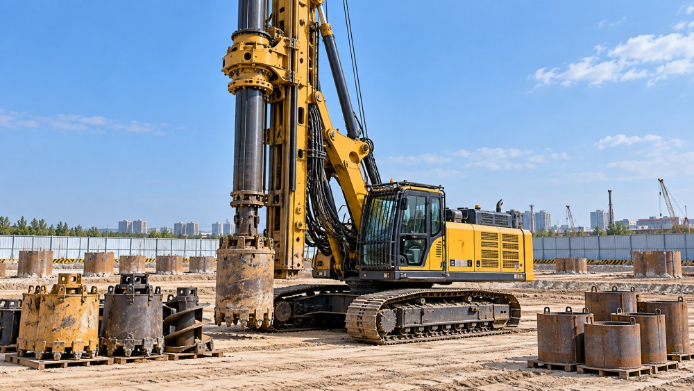
A lifecycle estimate needs a defined application, not just a machine model. A rotary bored piling rig, a driven piling system, and a continuous flight auger rig have different tooling, auxiliary equipment, wear mechanisms, and production constraints. Even two rigs with similar advertised torque may have different economics at the required diameter and depth.

Set a common operating basis that includes:

• Work requirements: pile type, diameter or section, depth, installation tolerances, and acceptance criteria.
• Ground conditions: expected soil and rock profiles, groundwater, obstructions, and casing requirements.
• Operating pattern: shifts, annual engine hours, expected project gaps, and relocation frequency.
• Ownership horizon: planned years of use and accumulated hours at disposal.
• Equipment boundary: rig, hammer or rotary attachment, tooling, power pack, and required support equipment.

The equipment boundary matters commercially. One quotation may include a working tool package, while another covers only the base machine. A lighter rig may also require additional support equipment for a particular installation method. Compare complete working configurations rather than headline prices.

Confirm technical suitability before calculating economic rankings. Lower hourly cost has little value if the machine cannot reliably deliver the specified piles under the expected ground conditions.

Build the estimate around cash flows, not accounting depreciation

For an undiscounted comparison, the basic calculation is:

Lifecycle cost = delivered and commissioned cost + operating costs + maintenance and repairs + other ownership costs + disposal costs − resale proceeds.

Delivered and commissioned cost should include freight, transport insurance, import duties where applicable, inland haulage, assembly, inspection, training, and the initial equipment package. Recoverable taxes should normally be separated from permanent costs, although their temporary cash-flow effect may still matter.

Recurring expenditure includes fuel or electricity, lubricants, filters, wear parts, scheduled servicing, repairs, labor, insurance, storage, and relocations. Include an initial spare-parts inventory as a cash outlay, but recognize its remaining value at the end of the assessment period where appropriate.

Do not add accounting depreciation to the full purchase price. Subtracting resale proceeds from acquisition cost already captures capital consumption in this simple model.

Financing requires a separate choice. An equipment-level economic comparison can exclude loan payments and discount future cash flows at an agreed rate. A financing affordability model instead tracks the deposit, repayments, interest, fees, and disposal proceeds, without also counting the full purchase price as a separate cash payment. Mixing these approaches double-counts capital.

For multi-year evaluations, discounted cash flow is more informative when spending schedules differ materially. Use a consistent price basis: nominal cash flows with a nominal discount rate, or constant-price cash flows with a real rate. If calculating a discounted cost per hour, discount both costs and productive hours consistently.

Separate engine hours from productive piling hours

Engine hours are useful for estimating fuel consumption and service intervals. They are not automatically the correct denominator for economic performance.

A rig can accumulate hours while idling, positioning, changing tools, handling casing, or waiting for another operation. Some of these activities are necessary parts of production; others reflect avoidable delays. Define “productive hours” consistently so one machine is not credited only for drilling time while another includes its complete installation cycle.

Cost per productive hour = lifecycle cost ÷ total productive hours over the ownership period.

Construct the hour forecast from a realistic work calendar. Deduct periods with no contracted work, planned servicing, expected breakdowns, and site constraints. Some losses overlap: a repair completed during an already-planned project gap does not create a second loss of productive time.

Keep technical availability separate from commercial utilization. Strong service support can reduce breakdown duration, but it cannot eliminate a lack of projects, delayed permits, or site-access restrictions.

Where machine productivity differs, cost per accepted pile or installed meter provides a stronger comparison. Divide the relevant total cost by accepted output under matched ground conditions and specifications. Include normal positioning, tooling changes, and expected rework. A low cost per operating hour can conceal a high cost per completed pile.

Estimate fuel, tooling, and repairs from the duty cycle

Rated engine power is not a fuel-consumption estimate. Request consumption information tied to identifiable operating conditions: installation method, load, ground type, depth, tool configuration, and idle share. Supplier figures without a defined duty cycle are weak inputs for a purchasing decision.

A practical fuel model separates working and idle consumption:

Fuel cost = [(working hours × working consumption) + (idle hours × idle consumption)] × delivered fuel price.

Include auxiliary power packs, compressors, or generators when required. For electrically powered equipment, account for the electricity supply arrangement, connection costs, and any relevant demand charges—not only the machine’s energy consumption.

Tooling deserves its own schedule. Cutting teeth, holders, drilling buckets, augers, casing components, hammer wear items, and wire ropes do not all wear in proportion to engine hours. Abrasive formations, obstructions, installation method, and handling practices can change replacement requirements.

Where credible information exists, estimate wear cost by installed meter, pile, or ground category, then reconcile it with the annual work mix. Avoid applying a soft-ground tooling allowance to a program containing substantial rock drilling.

For maintenance, obtain the service schedule and price the actual tasks. Include fluids, filters, technician travel, labor, and servicing time. Build major repairs separately around component condition, expected duty, and ownership duration; an annual percentage of purchase price can hide an expensive overhaul near the end of the holding period.

Used equipment needs a condition-based starting point. Inspection of hydraulic systems, mast and structural components, undercarriage, rotary drive or hammer, and service records can materially change the budget. An unverified maintenance history should increase the uncertainty allowance rather than justify a precise remaining-life forecast.

Translate service support into financial exposure

A warranty does not eliminate downtime cost. Parts may be covered while freight, travel, consumables, consequential losses, or certain labor charges are excluded. The contract must establish which expenses remain with the owner.

Ask for evidence behind service promises: local technician capability, stocked critical components, dispatch arrangements, diagnostic access, and lead times for items not held locally. Cross-border supply can add customs delays and transport uncertainty even when the manufacturer responds quickly.

Model plausible failure events rather than assigning an unsupported blanket downtime percentage. For each event, estimate repair expenditure, recovery time, replacement-equipment availability, and the unavoidable costs of the interruption.

Keep the treatment internally consistent. Reducing productive hours already raises calculated cost per productive hour. Add idle crew payments, replacement rental, or remobilization only where they represent additional costs not counted elsewhere. Lost contribution or contractual delay exposure can be shown separately as project risk; adding gross lost revenue to equipment cost would overstate the impact.

A worked comparison: when the higher price wins narrowly

The following figures are hypothetical assumptions, not market prices or performance benchmarks. Both machines are assumed to meet the same technical requirements and deliver comparable output per productive hour. The assessment covers six years, 9,000 engine hours, and 7,200 productive hours per machine.

Rig B costs $100,000 more initially but has a $45,000 lifecycle advantage under these assumptions. That advantage is modest enough to require scrutiny: if its net resale proceeds are $45,000 below forecast, the undiscounted cost advantage disappears.

The table excludes financing, tax effects, and project delay penalties. Equal productive hours are assumed only to isolate ownership and running-cost differences. If one rig produces faster, the comparison should be recalculated against a common output requirement, including the hours and resources needed to complete it.

Discounting could also change the ranking because Rig B requires more capital immediately while its savings and resale benefit arrive later.

Test the assumptions that could reverse the decision

A base-case total is not enough. Build downside and upside scenarios around the inputs with both substantial financial impact and weak evidence: annual utilization, ground-related wear, fuel consumption, major repairs, service delays, and residual value.

Change linked assumptions together where necessary. Lower utilization reduces fuel consumption and some wear, but insurance, storage, and capital costs remain. It may also change resale value. Applying the same percentage reduction to every cost category produces a misleading result.

Estimate resale proceeds for the expected age, hours, condition, configuration, and selling location. Deduct inspection, repairs needed for sale, commissions, transport, and other disposal expenses. Asking prices alone do not establish achievable proceeds.

Cross-border purchases also need currency scenarios for unpaid equipment balances, imported parts, and resale proceeds. Technical eligibility in the destination market—including applicable emissions, safety, and documentation requirements—should be confirmed before an apparently economical machine enters the final comparison.

Before committing, connect each material assumption to evidence: an itemized quotation, maintenance schedule, priced parts list, relevant consumption records, service agreement, inspection report, or supportable resale comparison. Record the source and uncertainty beside the number.

The strongest purchase case is not the spreadsheet with the lowest total. It is the technically suitable machine whose cost advantage survives realistic operating conditions—and whose remaining uncertainties can be bounded through evidence, contractual commitments, or a deliberate financial allowance.